The TornadoVM Programming Model Explained

Key Takeaways

• TornadoVM offers an API for parallel programming on modern hardware that tackles data parallel, task parallel and pipeline parallel applications.
• TornadoVM offers different API components to express parallel applications in Java, identify the methods to offload, and dispatch the application on the corresponding accelerators.
• Task-Graphs and Execution Plans are the main building blocks of TornadoVM applications, allowing developers to compose complex graphs of computations and interact with the TornadoVM runtime to enable/disable profiling, enable debugging, or enable dynamic reconfiguration to select the best possible accelerators for the compute graphs.

In this blog post, I will explain how developers can start programming with TornadoVM and interact with the TornadoVM runtime. I will explain the TornadoVM programming model and I will show an example from scratch that illustrates all the steps to be done to run on GPUs (or any other TornadoVM-compatible hardware).

Overview of the TornadoVM Software Stack

Let’s start with a general overview of the TornadoVM Software stack and the main components, as shown in the following Figure. At a high level, TornadoVM exposes an API for developers. This API contains the building blocks to be used by developers to express parallel applications, identify which methods to use and offload and run applications on GPUs and FPGAs. This API is the main content of this blog post.

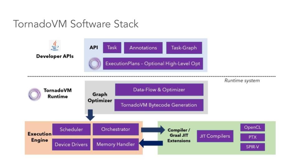
Under the hoods, the TornadoVM runtime system and the Just-In-Time compiler, optimise, compile and dispatch the input application on heterogeneous hardware. We will not go into the details of the runtime system in this tutorial, but in a nutshell, the TornadoVM JIT compiler extends the GraalVM JIT compiler to offload Java code to low-level GPU-friendly code, such as CUDA, OpenCL and SPIR-V. Then, the TornadoVM runtime takes care of data migration, data handling and execution of the application for the target hardware. Thus, in a way, TornadoVM is a full-package solution that is not only used for programming on modern hardware but also for orchestrating, running, and optimising a subset of Java programs on heterogeneous hardware.

How do we start programming?

So, let’s focus now on the API level and how developers can start using TornadoVM to program their applications. To understand the main ideas behind each API component in TornadoVM, we need to think about the following aspects:

1. How do we represent parallelism, in a programming language that was not primarily designed for parallelism and modern hardware? Note that, there are different types of parallelism, such as data-parallelism, task-parallelism and pipeline-parallelism, and we would like to run a subset of Java programs on explicit parallel hardware, such as GPUs. Thus, ideally, we would like an API to express these types of parallelization in our programs in an easy manner, and be able to dispatch our parallel programs on a wide diverse of modern hardware, such as GPUs, FPGAs, RISC-V accelerators, etc.
2. How do we identify which functions (or methods) to offload? We usually have large programs with hundreds of classes and thousands of methods, but how do we select the methods to be offloaded (to be transformed and migrated to the target accelerator)?
3. How do we run on parallel hardware? And how do we profile, get the results, etc?

The TornadoVM API tries to tackle all these questions with different API components. Let’s discuss this briefly one by one.

1. Representing Parallelism

There are two ways to express parallelism with TornadoVM, and developers can choose one or the other:

1. Via annotations in the source code: Annotating Java for-loops with the @Parallel annotation and reduction parameters with the @Reduce annotation for those loops that can be parallelisable. This means that, if the loop does not have data dependencies, we can add the @Parallel annotation to indicate to the TornadoVM compiler and runtime system that the loop/s can be parallelisable, and, therefore, the JIT compiler can perform the corresponding code transformations to convert Java sequential loops into explicit parallel loops. It is also possible to add nested parallel loops. This API is convenient for non-GPU/FPGA experts to get easier and quicker access to hardware accelerators.

2. Via an explicit parallel kernel API. Developers use the KernelContext API. This second API style is a lower-level API compared to the annotations, and it is more similar to OpenCL and oneAPI to program explicit parallel kernels. The use of the parallel kernel API is sometimes more convenient for developers who are already familiar with OpenCL, oneAPI or CUDA and want to port existing kernels into TornadoVM. By using the KernelContext API, the developers can access shared memory (or local memory), and barriers, and control the thread dispatcher of the entire kernel.

In this post, we will focus on the first option, using the TornadoVM annotations for the for-loops. Let’s see this in practice through an example. Let’s say we want to initialise an array of floating point numbers (in fp32) and perform some computations with this array. Thus, let’s code two methods for 1) initialization of an array; and b) perform a computation (e.g., compute the SQRT function from the Math library):

public class MySample { 
    public static void init(FloatArray array) {
        for (int i = 0; i < data.getSize(); i++) {
            array.set(i, i * 2);
        }
    }

    public static void computeSqrt(FloatArray array) {
        for (int i = 0; i < data.getSize(); i++) {
            float value = array.get(i);
            array.set(i, Math.sqrt(value));
        }
    }

    public FloatArray compute(FloatArray array) {
        init(array);
        computeSqrt(array);
        // do something else
        // ...  
        return array;
    }
}

A few things to highlight regarding this code snippet:

1. We see a data type called FloatArray. This data type is provided by the TornadoVM API, and it contains (as the name suggests) an array of floating point numbers (fp32). The array is stored off-heap using the Java Panama Memory API. The TornadoVM API provides types for 1D, 2D and 3D arrays, as well as image types, volumes and explicit vector types (e.g., Float8: link). For this tutorial, we are going to stay with our FloatArray, but feel free to scan the API and Collections of TornadoVM to see all the supported types.

2. We see that each method returns void, and the inputs and outputs are passed as arguments to the methods. This is intentional since the TornadoVM will offload each of the Java methods to run in parallel on the target device (e.g., a GPU). Since the target hardware of TornadoVM allows developers to run many threads (usually > 1000s threads), it would be almost impossible to determine which thread/s returns a value from the entire method efficiently. Thus, we provide the method in a more “Tornado”-friendly way to approach the next step (use the annotations in the for-loops). As a side note, other parallel programming models, such as OpenCL, CUDA and oneAPI, also provide similar rules to code parallel kernels (return void).

We introduce the @Parallel annotation for parallel loops of the methods we want to offload. When using the annotation, it is the responsibility of the developer to include the @Parallel annotation in the loops that do not have data dependencies. This is a similar programming model to OpenMP, or OpenACC. This annotation will indicate the TornadoVM compiler that we want to run the whole loop in parallel using many threads.

But, how many threads?: The number of threads depends on the loop bound of the annotated loop. But this is transparent to Java developers, and the TornadoVM runtime and the JIT compiler work together to set these values.

Going back to our example, let’s add the annotations for the two methods we potentially want to offload: the init and the computeSqrt methods.

public class HelloTornado { 
    public static void init(FloatArray array) {
        for (@Parallel int i = 0; i < data.getSize(); i++) {
            array.set(i, i * 2);
        }
    }

    public static void computeSqrt(FloatArray array) {
        for (@Parallel int i = 0; i < data.getSize(); i++) {
            float value = array.get(i);
            array.set(i, TornadoMath.sqrt(value));   // << Use TornadoMath class instead
        }
    }

    public FloatArray compute(FloatArray array) {
        init(array);
        computeSqrt(array);
        // do something else
        // ...  
        return array;
    }

Furthermore, for this step, we transform the Math.sqrt into TornadoMath.sqrt. TornadoVM offers a math library, similar to Java. The reason for having this library is that, for some GPU/FPGA devices, double (fp64) types are not supported (for example on Intel ARC GPUs, or the latest Intel HD graphics). However, we can still compute sqrt or many of the math functions using less precision, such as in fp32 (float in Java), or even less. To allow this integration, TornadoVM offers this API that the JIT compiler can understand and provide the correct replacements using the narrower types (e.g., fp32 or fp16).

Besides, there is another reason why you might want to use the TornadoMath library for your applications when running on GPUs, and that’s performance. CPUs, usually offer the same performance when computing fp32 and fp64 operations. However, this is not usually the case for current GPUs. For example, while you can compute operations in double (fp64) precision on NVIDIA GPUs, there are usually fewer functional units per GPU thread in fp64 compared to fp32. And this means that, if operating in fp64, CUDA threads need to share the functional units. To give an example, using the RTX 4090 GPU, the ratio is 1:64. Thus. be careful! In GPU programming, think twice before you operate using double data types.

Now, let’s move on to create our compute graphs.

2. Identifying the Java Methods to Offload

TornadoVM offloads code at the method level (similar to the JIT compiler in Hotspot). To specify which method/s to offload, TornadoVM offers a Task-Graph API, in which each node in the graph represents a task. Besides, we add the data inputs and outputs of our computation to the graph. This is useful for the TornadoVM runtime, which needs to perform data migration between the host (main CPU) and the accelerator (e.g., the GPU), since in many cases, the computing system does not share the same memory for both accelerators and the CPU.

To continue with our example, we build the Task-Graph as follows:

public class HelloTornado { 
    public static void init(FloatArray array) {...}

    public static void computeSqrt(FloatArray array) {...}

    public FloatArray compute(FloatArray array) {
        TaskGraph graph = new TaskGraph("graph")  
          .transferToDevice(DataTransferMode.EVERY_EXECUTION, array)
          .task("init", HelloTornado::init, array)
          .task("compute", HelloTornado::computeSqrt, array)
          .transferToHost(DataTransferMode.EVERY_EXECUTION, array);
        return array;
    }

We see that, for creating and defining all data and tasks of our computation, we use mainly three methods from the Task-Graph API:

1. transferToDevice: define all objects to be copied to the target accelerator. We also define a mode for each of the objects. In this case, we specify that the array object must be transferred every time the whole graph is executed. This is because we can execute the graph multiple times. If the mode is declared as FIRST_ITERATION , the array is copied only the first time that the whole graph is launched to the target accelerator. This is useful if we want to define read-only data.
2. task: This is the method identification. To identify uniquely every method, we give a name. This name is useful to check with the profiler, change the device at runtime, etc, as I will show in the next step. The next parameter of this method is the reference to an existing Java method. This could be a lambda expression, an instance method, or a static method. In our example, we use a reference to a static method. We can define as many tasks as we want, and, as soon as they are accessible from the class that instantiates the task graph, each referenced method could be located in different Java classes.
3. transferToHost: defines the data objects in which we expect the output of our computation. This could be one or many objects. Additionally, we pass a mode. Usually, we want the output to be transferred to the host right after the execution of a task graph has finished. However, in some cases (e.g., iterative algorithms), we want to execute a graph multiple times and only transfer the data at the end. In this case, we could also define data to be transferred UNDER_DEMAND and use another data structure (called TornadoExecutionPlan) to copy data under demand.

Note that the Task-Graph is never executed. It only defines which method/s, and which object/s to use. To execute a Task-Graph, we need to instantiate an object of type TornadoExecutionPlan.

3. Deploying and Running Task-Graphs

We are almost done. To execute a task graph, we need to instantiate an execution plan. The execution plan, receives, as an argument, a snapshot of an existing task graph.

Wait, a snapshot? what is this?

A snapshot is an object that contains an immutable task graph, which in turn, is a task graph that cannot be changed (e.g., add new tasks, or add new data). This is by design to avoid changing the task graph (meaning appending more tasks or adding more data) while we execute code on the GPU.

Let’s go back to our example and create an execution plan from the graph object:

TornadoExecutionPlan plan = new TornadoExecutionPlan(graph.snatshot());

And now, we can call the execute method:

plan.execute())

Done! If we do not specify anything else, the execute method in a blocking call, and it will optimise, compile and run the whole task graph on the default device.

For reference, this is the entire code of our example:

public class HelloTornado { 
    public static void init(FloatArray array) {
        for (@Parallel int i = 0; i < data.getSize(); i++) {
            array.set(i, i * 2);
        }
    }

    public static void computeSqrt(FloatArray array) {
        for (@Parallel int i = 0; i < data.getSize(); i++) {
            float value = array.get(i);
            array.set(i, TornadoMath.sqrt(value));   
        }
    }

    public FloatArray compute(FloatArray array) {
        TaskGraph graph = new TaskGraph("graph")  
            .transferToDevice(DataTransferMode.EVERY_EXECUTION, array)
            .task("init", HelloTornado::init, array)
            .task("compute", HelloTornado::computeSqrt, array)
            .transferToHost(DataTransferMode.EVERY_EXECUTION, array);
        TornadoExecutionPlan plan = new TornadoExecutionPlan(graph.snatshot());
        plan.execute())
        return array;
    }

Interacting with the Dispatcher

We can also change the default decisions of the TornadoVM runtime, and perform some actions (e.g., enable the profiler, change the hardware accelerator, enable dynamic reconfiguration, etc). The TornadoVM Execution Plan follows a builder pattern to specify all these actions.

For example, to change a device:

int driverIndex = 0;
int deviceIndex = 1;
TornadoDevice device = TornadoExecutionPlan.getDevice(driverIndex, deviceIndex);
plan.withDevice(device)
    .execute();

And we can execute again, without the need to build a new task-graph.

If we want to enable dynamic reconfiguration (a feature of TornadoVM to discover the best device depending on a policy), we can enable it as follows:

plan.withDynamicReconfiguration(Policy.PERFORMANCE, DRMode.PARALLEL)
    .execute();

In this call, we specify that we want to select the best device in terms of performance, and the TornadoVM should evaluate all permutations in parallel. What this API call will trigger, is to compile and run for all hardware accelerators available in our system, and choose the best device that follows the policy we specified. Cool, isn’t it? If you want to know more about dynamic reconfiguration, this paper contains more details.

There are more methods in the TornadoExecutionPlan class. We covered just two of them. If you are interested, I invite you to read the documentation and the examples. Additionally, I recorded a video showing, step by step, some of these functions in action.

Summary

In this post, we have explained the basics of the TornadoVM programming model and the main API blocks. With these tools, developers can start integrating these components into their applications and start accelerating portions of the Java programs on hardware accelerators, such as GPUs.

If you want to know more, I invite you to explore the example suite in TornadoVM to get an idea of the types of applications that can be expressed using the TornadoVM API with more complex use cases.